
The idea of using mathematical skills and advanced analytical techniques to help improve NBA basketball teams has created controversy throughout the basketball community over recent years. Some individuals, such as former NBA player Charles Barkley, believe that analytics do not have an effect on helping teams win basketball games; it is up to the coaching staff and professional basketball players to improve their performance. In contrast, others, such as Dallas Mavericks owner Mark Cuban, claim using analytical techniques helped assess the efficiency and effectiveness of their NBA team, and allowed the coaching staff to make decisions to put the organization in the best possible chance to be successful.
Predictive data analytics uses various types of data to solve problems and assist others in making better decisions. However, in order for analytics to be effective, it is extremely important to ask the right questions and order to interpret the data accurately and to solve problems correctly.
Background: Data Analytics In Basketball, Data Mining, & Decision Trees
Data Analytics In Basketball
Recently in basketball, several statistical techniques are used to track almost every aspect of the game. The number of points scored per game, the stats of each individual player, and the team efficiency percentages are just a few examples of key information that is logged during the games of the NBA season. Whether it is as simple as keeping track of the score each game, or as complex as finding a player's efficiency rating (PER), almost every NBA organization has an analytics team that uses numerous technologies and techniques to record various numerical data and advanced metrics. Once the analytics staff watch the basketball games and collects a thorough set of raw data, they are able to look for patterns in the data, organize it, analyze it, and report their findings to the coaching staff and players in hopes that their work will improve the team’s success.
Data Mining And Predictive Analysis
The process of analyzing and extracting large raw datasets to generate new information is called data mining. In order for these basketball analysts to find patterns and extract information from these complicated datasets for their teams, they typically use various algorithms to help them go through the numerical metrics. An algorithm is a procedure that uses a precise set of steps to solve mathematical problems and computation. They are great for finding efficient ways to do complicated calculations and finding shortcuts to solve complex problems faster than just using the standard math principles of addition, subtraction, multiplication, and division.
Decision Tree Algorithms
There are several algorithm techniques that can be used to organize these large, raw basketball datasets during the data mining process. For this essay and my model, we are going to use a decision tree, a popular, modern classification algorithm that is used in data mining and machine learning. Decision trees are tree-shaped classification diagrams that divide and branch data into smaller sub-datasets based on the descriptive attributes you are analyzing; it continues to break down the data until the data points fall into a label that cannot be further broken down.
They solve classification problems by predicting categorical outcomes using numeric and categorical variables as input. If a basketball analyst were to set and train the decision tree to test certain characteristics, it would be able to show basketball analysts how one particular characteristic or action can lead to a certain outcome. The advantage of using a decision tree algorithm is that the steps in creating this model are fast and simple, and it is also easy to comprehend and analyze.
As seen in the diagram below (Figure 1), a decision tree model consists of several nodes and branches. A given situation starts at a decision node called the root node, which starts the whole algorithm; the information is then divided and organized into different nodes, depending whether data contained the set variable the root node asked for or not. The new sub-nodes created from the root node are called decision nodes; they contain and ask for different variables, causing the information to diverge into further possibilities. The branches of the decision tree represent the flow of the information from the node asking the question to the answer and next node. Once a node can no longer break down into further possibilities, a pure final answer is found; the final value is termed as the leaf node.
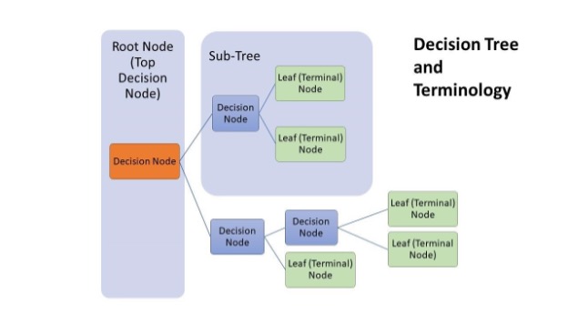 Figure 1: Diagram of a decision tree algorithm with labels (Poojari).
Modeling The Predictive Power Of Team Performance Metrics
Data And Variables
Before I could start building my decision tree models, I first needed to choose what variables I was going to classify my data and use for my root node and decision nodes. Because I am manually structuring a decision tree algorithm, it is recommended that I should not use more than three variables in the single algorithm, because the information expands quickly and exponentially. Therefore, after examining several different team stats recorded in the NBA, I decided on four total attributes: field goals made per game (FGM), rebounds per game (REB), turnovers per game (TO), and effective field goal percentage per game (EFG%).
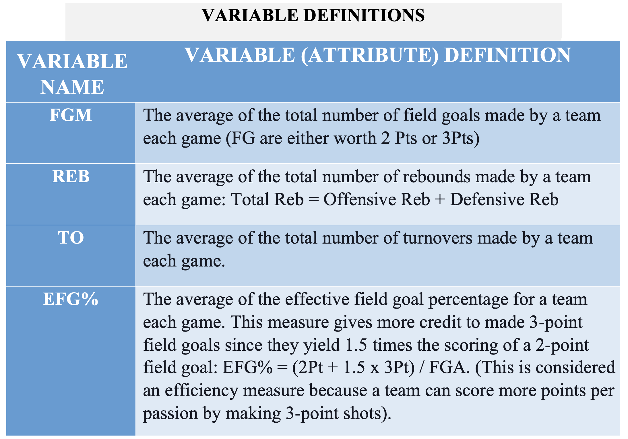 Table 1: The NBA team attributes used as my variables for my decision tree models. (Basketball Breakthrough)
Once I selected the variables, I researched data to use in the algorithm, as well as a reference data to set used to sort the data. The data used was the team data for all NBA teams in the 2018-2019 season. I chose this season because it was the last full, normal season before COVID-19. As for the split variables or attributes, I decided to use the average team performance metrics of all NBA championship-winning teams from the 10 years prior to the 2018-2019 season. I determined that the team metrics from the previous championship teams would make a great standard for my models because each of these teams qualified for the playoffs for the season in the year when they won the championship. The summary metrics used in my model are shown in the table below (Table 2).
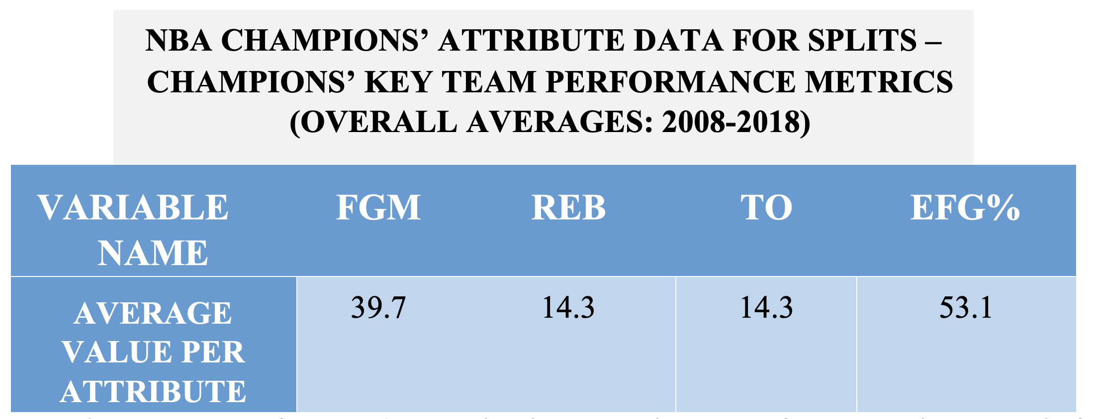 Table 2: The averages from NBA champions’ team attribute data for each variable used in for my decision tree models (NBA Stats)
As shown in Table 2 above, the overall average for each team metric for the championship teams is listed (see Table 1A in the appendix for the raw data). Next, I use the same team performance metrics for every team from the 2018-2019 NBA season, as well as created a variable that denoted whether each team made the playoffs or not (see Table 2A in the appendix for the raw data.).
Building The Model
The next step is to construct my decision tree models used to test my research question.
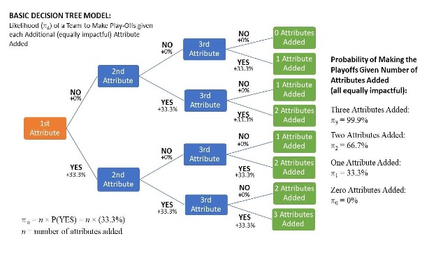 Diagram 1: A basic decision tree model for predicting whether teams make the playoffs.
To understand how the decision tree models work, consider the basic model above (Diagram 1). In this model, I assume the more attributes a team has, the higher chance to make the playoffs; and, each attribute adds the same impact of going to the playoffs. As they move through the decision tree and go through each “yes” branch, their probability of making the playoffs increases by 33.3 percent. In contrast, if they go through the “no” branch, their probability of making the playoffs does not increase. This process repeats itself at every decision node until the algorithm reaches the leaf nodes, which shows how many attributes a team has.
Teams with three attributes have a 99.9 percent chance at making the playoffs, those with two attributes have a 66.6 percent chance, those with one attribute have a 33.3 percent chance, and those with no attributes have no chance at making the playoffs.
However, in the situation I am modeling, I do not know the actual impact of each attribute; I have to estimate it. Therefore, the ordering of the variables used to split the data is extremely important. To determine the order of the team attributes in the decision tree, I calculate the GINI values of each attribute. The GINI value informs me which attribute gives me the highest information gain for the algorithm when predicting the results.
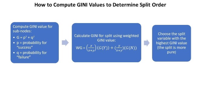 Figure 2: Explaining how to solve for the GINI value and how it helps determine the order for the decision tree algorithm. (Poojari)
As shown above (Figure 2), the equation to compute the final weighted GINI value for a specific attribute is written below:

where:
- ‘x’ is the number of teams that followed the “yes” branch
- ‘y’ is the number of teams that followed the “no” branch.
- G(Y): the GINI value for the teams that followed the “YES” branch
- G(N): the GINI value for the teams that followed the “NO” branch
Math Calculations
The detailed mathematical calculations and terminology are shown below. The table below shows the definitions of the terminology and variables used in the GINI calculations
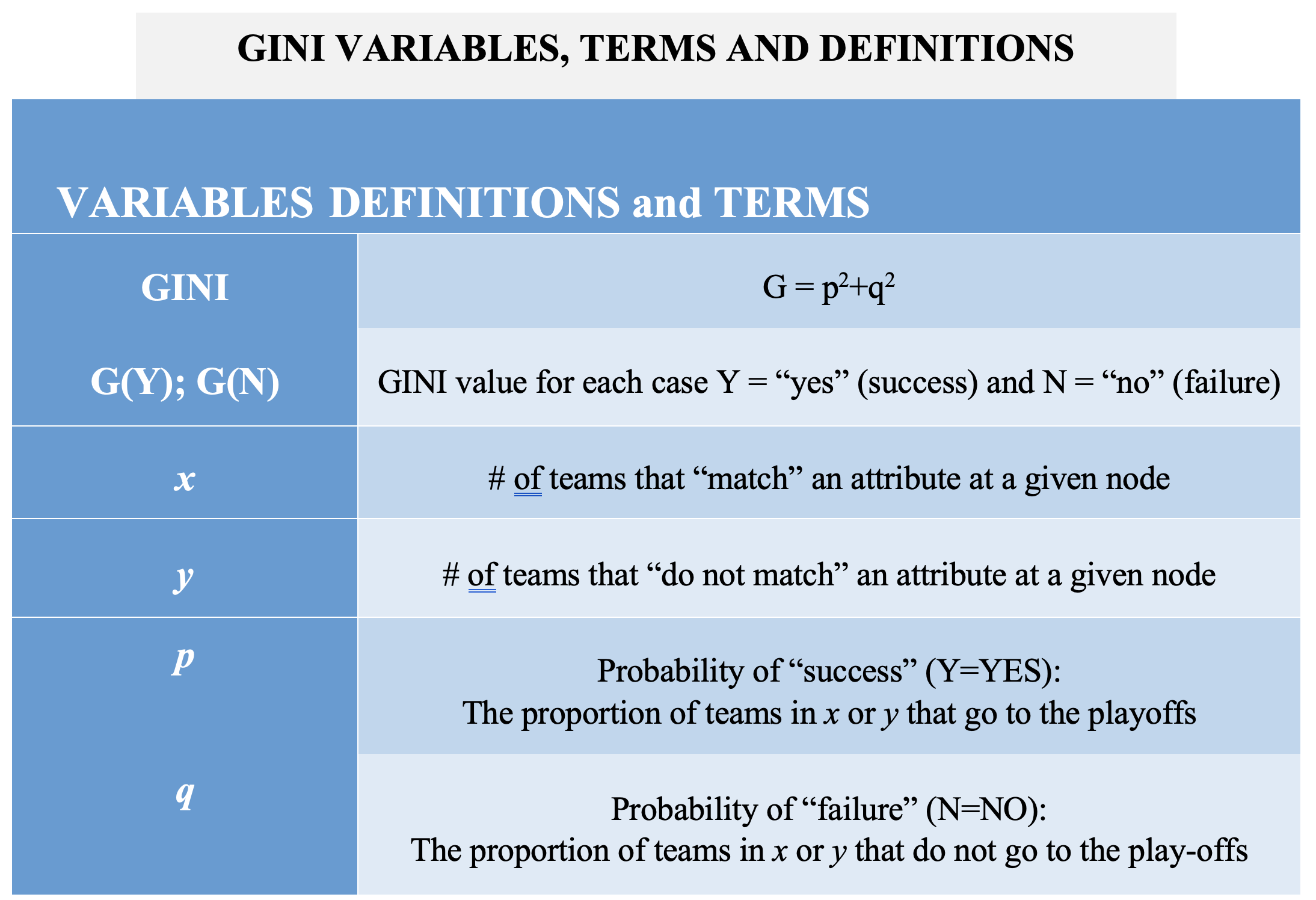 Table 3: Terminology and variable definitions for formulas to compute GINI values.
Below are the detailed calculations for the GINI values used to select the root node and determine the sort order for each decision tree model.
FGM ≥ 39.7
Below are the calculations for the GINI and weighted GINI values for the attribute FGM ≥ 39.7:

REB ≥ 43.0
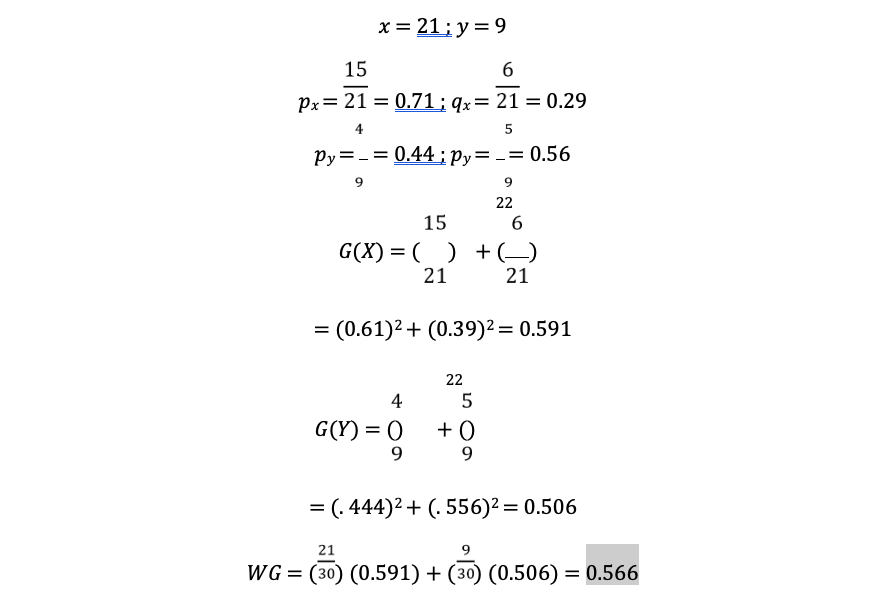
Below are the calculations for the GINI and weighted GINI values for the attribute REB ≥ 43.0:
TO ≤ 14.3
Below are the calculations for the GINI and weighted GINI values for the attribute TO ≥ 14.3:
EFG% ≥ 53.1
Below are the calculations for the GINI and weighted GINI values for the attribute EFG% ≥ 53.1):
The table below gives a summary of the different GINI values I compared to determine the root node for each of my decision tree models and the order to split them further (Table 4).
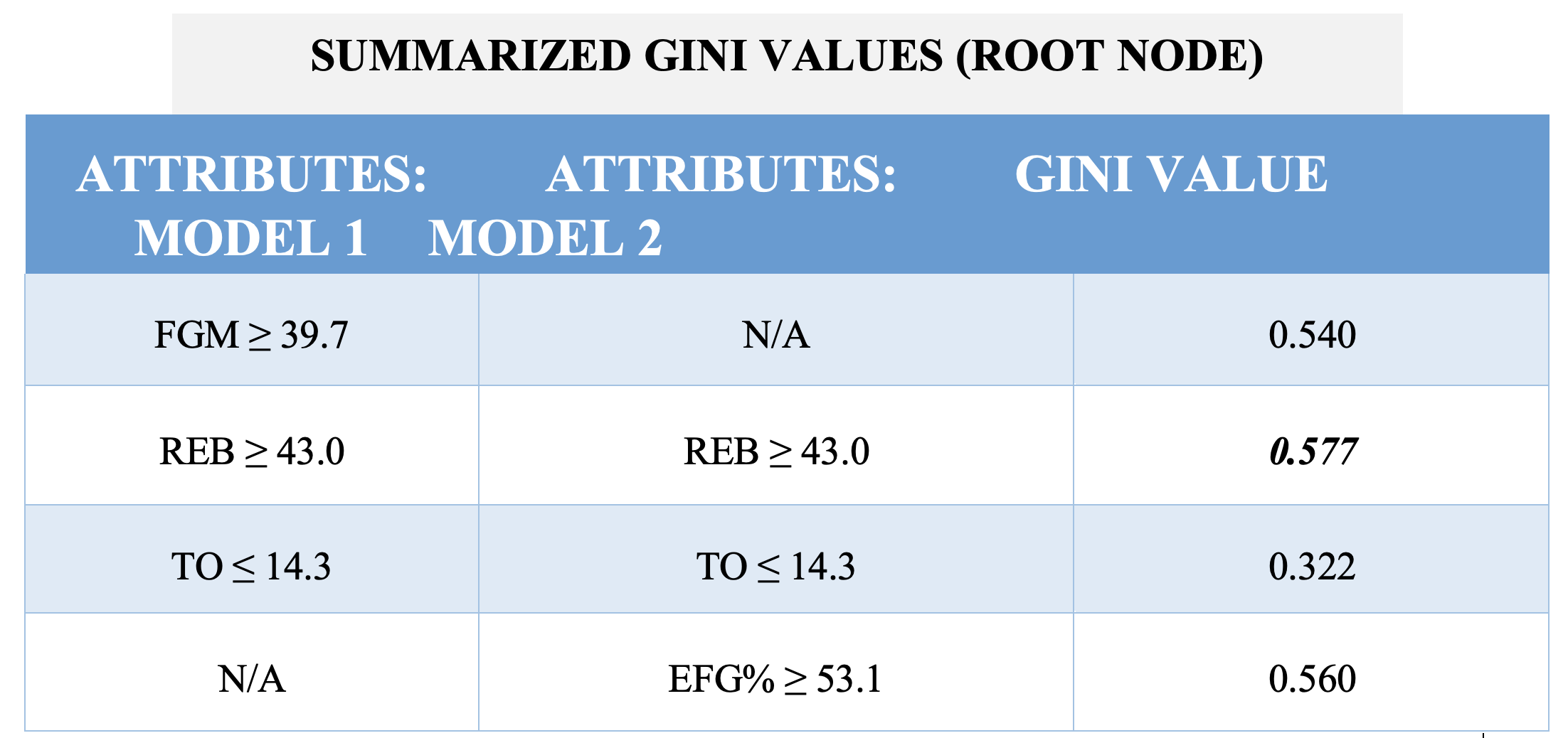 Table 4: GINI values by team attribute, and the selected root node. The weighted GINI value in boldface type is biggest, so requires REB to be the root node for both Model 1 and Model 2.
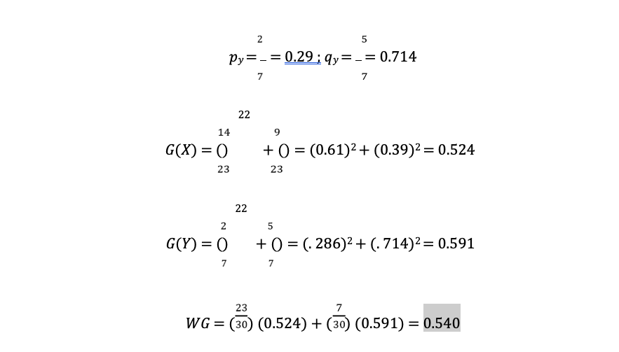
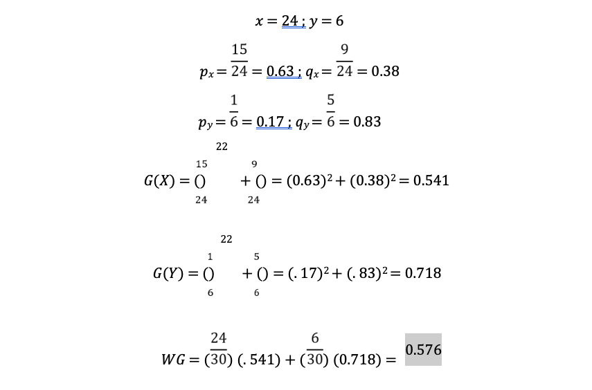
After selecting the variable for the root note, I calculated the weighted GINI values for the last two variables for each model, respectively. The calculations for these two cases are shown below and the summary of the values are shown in the next table below (Table 5).
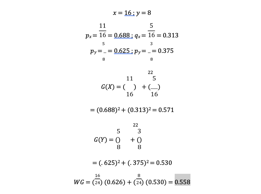
Below are the calculations for the weighted GINI value used to select the order for the remaining decision nodes in Model 1 and Model 2. Since there are 24 teams that “answer ‘YES’ at the root note (REB ≥ 43.0), this means the GINI values for the second node is calculated for only 24 teams:
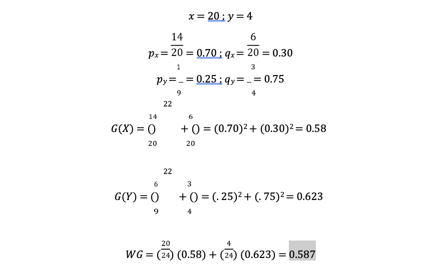
FGM ≥ 39.7
Below are the calculations for the GINI and weighted GINI values for the attribute FGM ≥ 39.7.
TO ≤ 14.3
Below are the calculations for the GINI and weighted GINI values for the attribute TO U+02265 14.3:
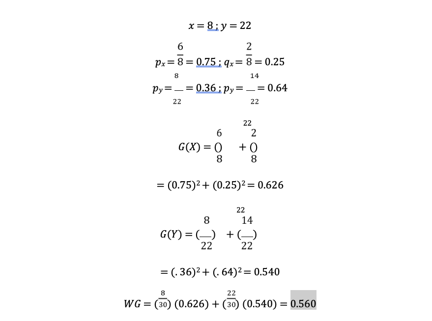
EFG% ≥ 53.1
Below are the calculations for the GINI and weighted GINI values for the attribute EFG% ≥ 53.1):
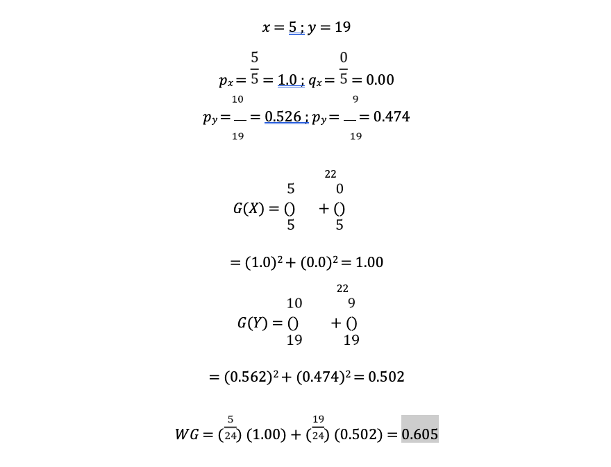
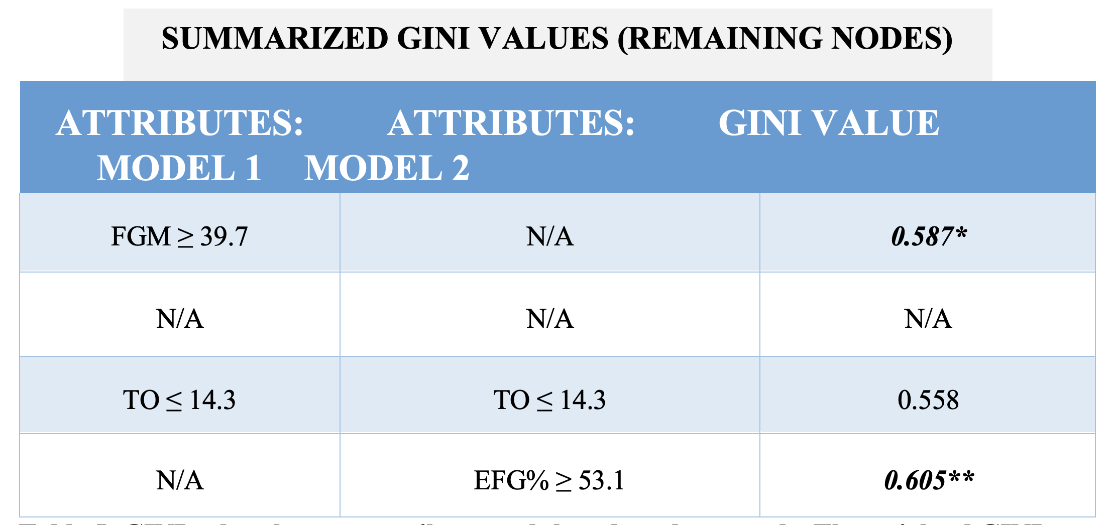 Table 5: GINI values by team attribute, and the selected root node. The weighted GINI value in bold face type is biggest, so requires FGM to be the second split variable in Model 1 and EFG% to be the second split variable in Model 2.
Model 1 and Model 2
In the first model, I used the variables FGM, REB, and TO. As shown on Table 4, REB has the highest weighted GINI value compared to the other two, so that is the root node for this decision tree. For the second split, I recalculated the weighted GINI value for both FGM and TO at the second decision node. As shown on Table 5, FGM had the higher GINI value, so this attribute is used for the second split. For the last split, I do not have to calculate the GINI value again because TO is the only attribute remaining to be added onto the model.
After finalizing the first decision tree model, I wanted to see if the model could produce a more accurate prediction, so I developed a second model. In the second model, I decided to use EFG%, REB, and TO, and did not use FGM. I decided that a variable that is an efficiency measure might be a better predictor in the model than a variable that is a basic measure of total field goals made. As shown on Table 4, REB, again, has the highest weighted GINI value compared to the other two attributes, so that is the root node for this decision tree. For the second split, I recalculated the weighted GINI value for both EFG% and TO. As shown on Table 5, EFG% had the higher weighted GINI value, so this attribute is used for the second round of decision nodes. Again, I did not have to calculate the weighted GINI value for TO again. In the next section, I discuss the specific findings from both models.
Results & Analysis
Model Results
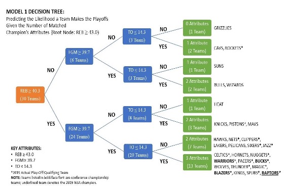 Diagram 2: The results of the first decision tree, showing how many attributes each team had during the 2018-2019 season.
The diagram above (Diagram 2) displays the results after the first decision tree model organized all 30 teams from the 2018-2019 season. The decision tree algorithm said 13 teams possessed all three attributes equal to or greater than those of the NBA champions. 12 teams possessed two of the three attributes, four teams possessed one of the three attributes, and one team possessed none of the attributes from the model.
Looking at the model, if I were to assume that all variables carry the same importance for making the playoffs, the first model does a decent job predicting the probability of teams making the playoffs with either three, two, one, or no attributes. 10 out of 13 (76.9%) teams that possessed all three attributes made the playoffs during the 2018-2019 season, leaving a 23 percent difference compared to what the basic model predicted (see Figure 2). Five out of the 12 (41.6%) teams that had two attributes made the playoffs, leaving a 25 percent difference compared to what the basic model predicted. One out of four (25%) teams that possessed only one attribute made the playoffs, leaving an 8.3 percent difference compared to what the basic model predicted. Finally, the one team that possessed none of the attributes did not make the playoffs, which is exactly what the basic model predicted.
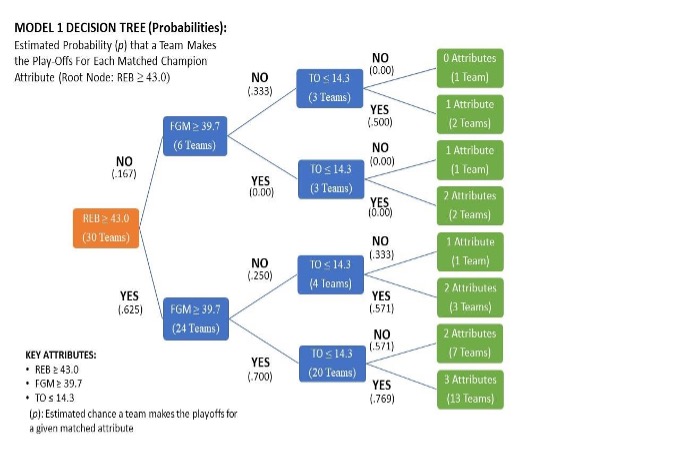 Diagram 3: How the probability of teams making the playoffs is estimated based on which attributes each team had (for Model 2)
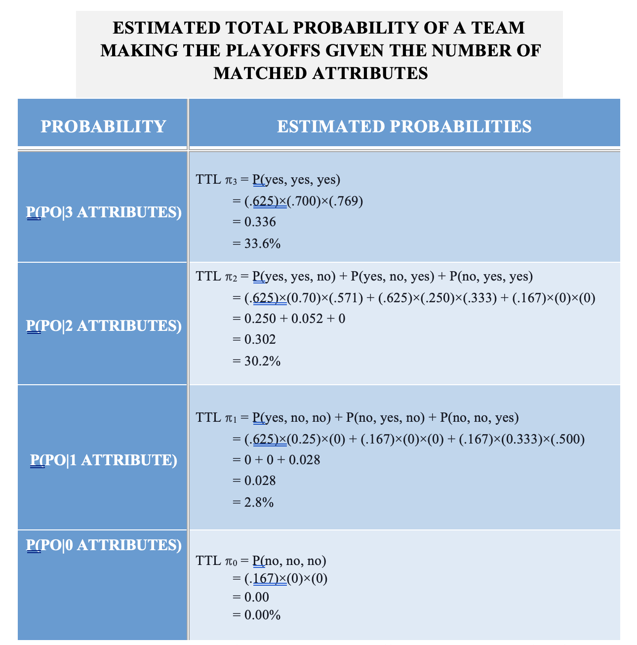
Diagram 3 and Table 6 above show how I calculated the estimated probability of teams getting into the playoffs given the number of performance attributes that matched or were better than the NBA champions, assuming that each attribute does not carry the same importance for making the playoffs. The probabilities were calculated by multiplying the fraction of teams that took a specific route that led them to have three attributes, two attributes, one attribute, or no attributes. Because there are multiple ways teams can end up with one or two attributes, I added the individual probabilities together to get a total value that represents the probability of making the playoffs if teams have one attribute or two attributes. According to Table 6, teams have a
33.6 percent chance to make the playoffs if they possessed all three attributes as the previous NBA champions. Teams with two attributes have a 30.2 percent chance, teams with one attribute have a 2.8 percent chance, and those who possess none of the attributes have no chance at making the playoffs. Overall, although the first decision tree model did an alright job at sorting out all 30 teams, the estimated probability compared to the actual results of the 2018-2019 were not as accurate as it could be.
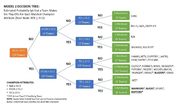 Diagram 4: The results of the second decision tree model, showing how many attributes each team had during the 2018-2019 season.
Moving on to the second model, after substituting FGM with EFG%, Diagram 3 shows that the decision tree algorithm said four teams possessed all three attributes equal to or greater than those of the NBA champions. 16 teams possessed two of the three attributes, nine teams possessed one of the three attributes, and one team possessed none of the attributes from the model.
Looking at the model, if I were to assume that all variables carry the same importance for making the playoffs, the second model does a noticeably better job than the first model at sorting which teams make the playoffs versus which teams do not. 100 percent (100%) of the teams that possessed all three attributes made the playoffs during the 2018-2019 season, leaving only a 0.01 percent difference compared to what the basic model predicted (see Figure 2). Eight out of the 16 (50%) teams that had two attributes made the playoffs, leaving a 16 percent difference compared to what the basic model predicted. Two out of nine (22.2%) teams that possessed only one attribute made the playoffs, leaving a 11.1 percent difference compared to what the basic model predicted. Finally, the one team that possessed none of the attributes did not make the playoffs, which is exactly what the basic model predicted.
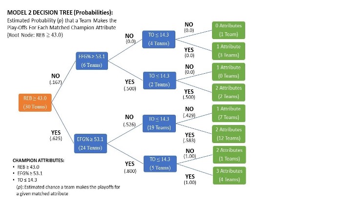 Diagram 5: How the probability of teams making the playoffs is estimated, based on which attributes each team had (For Model 2).
 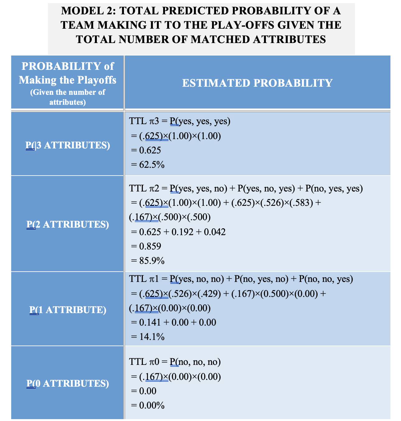 Table 7: Estimated probability of getting into the playoffs given the number of performance metrics that match the champions’ key team metrics (for Model 2).
Diagram 5 and Table 7 above show how I calculated the estimated probability of teams getting into the playoffs given the number of performance attributes that matched or were better than the NBA champions, assuming that each attribute does not carry the same importance for making the playoffs. I used the same calculating process as when I calculated the estimated probability for my first model. According to Table 7, teams have a 62.5 chance to make the playoffs if they possessed all three attributes as the previous NBA champions. Teams with two attributes have an 85.9% percent chance, teams with one attribute have a 14.1 percent chance, and those who possess none of the attributes have no chance at making the playoffs. Even though the results of the second decision tree model were not identical to the actual results of the 2018-2019 season, it still did a better job than the first decision tree model at predicting the probability of what teams make the playoffs based on the performance metrics each team possessed.
Conclusion
To conclude, I learned how to use data mining and decision tree algorithms to try and predict NBA teams that make the playoffs versus teams that do not. Although my models had their strengths and weaknesses, they did a relatively decent job at predicting the estimated probability of which teams make the playoffs, given the team performance metrics they produce. Also, I noticed that the second model improved because I replaced a basic team performance metric with an efficiency team performance metric. Efficiency team performance stats consider more variables and metrics that take place during a basketball game. With that being said, it would be interesting to compare results of two decision tree algorithms, where one contains only basic team performance metrics and the other contains only efficiency team performance metrics.
Works Cited
"Basketball Statistics Definitions." Basketball Breakthrough. Web. 12 Mar. 2021."Decision Tree." Decision Tree. Web. 12 Mar. 2021.
"How NBA Analytics Is Changing Basketball: Merrimack College." Merrimack College Data Science Degrees. 25 June 2020. Web. 12 Mar. 2021.
"Inspirationalbasketball.com." Web. 12 Mar. 2021.
M, Prachi. "What Is Decision Tree Analysis? Definition, Steps, Example, Advantages, Disadvantages." The Investors Book. 07 Mar. 2020. Web. 12 Mar. 2021.
MayaHeee, Lyla, and Silvia Valcheva. "10 Top Types of Data Analysis Methods and Techniques." Blog For Data-Driven Business. 28 May 2020. Web. 12 Mar. 2021.
Poojari, Devesh. "Machine Learning Basics: Decision Tree from Scratch (part I)." 01 May 2020. Web. 12 Mar. 2021.
Russell, Deb. "Are We Living in the Age of Algorithms?" ThoughtCo. Web. 12 Mar. 2021.
Sethneha. "Entropy: Entropy in Machine Learning For Beginners." Analytics Vidhya. 24 Nov. 2020. Web. 12 Mar. 2021.
Steve, James Kerti, Josh Url, Will, Larry Coon, Andrea, On the Importance of Frames of Reference | Analytics Game Says:, Basketball Analytics: Reflections and Reservations | Between the Lines Says:, and Analytics: The Future of the NBA – Eric's Basketball Blog Says:. "What Basketball Analytics Really Means." Basketball Scouting Guide. 29 Dec. 2020. Web. 12 Mar. 2021.
"Teams Traditional Stats." NBA Stats. Web. 10 Mar. 2021.
Theobald, Oliver. Machine Learning for Absolute Beginners. (Second Edition) ed., Oliver Theobald, 2017.
Yadav, Ajay. "DECISION TREES." Medium. Towards Data Science, 11 Jan. 2019. Web. 12 Mar. 2021.