The Purpose of this Study
This study looks at the effect of football spending among Power Five programs on wins for their respective teams. I took spending data from Knight-Newhouse College Athletics Database[i] and win totals for 47 Power Five teams (collected from ESPN website[ii]) and analyzed the relationship between the two using the R Project for Statistical Computing. I looked at data from 2005 (the year FBS teams moved to a 12-game season) to 2022 (except for total football spending data in 2021, which was unavailable). I also did not include data for the 2020 football season, as it seemed not representative due to the many unusual variables of the pandemic. The four categories of Universities’ football spending analyzed in this study are Recruiting, Facility Investment, Coaches’ Salaries, and Total Football Spending (which includes the above categories plus student aid, competition guarantees, game expenses/travel, medical and support, and administrative compensation). I also looked at the total revenue gained from football programs, which includes many sources: TV deals, merchandise, and ticket sales. One apparent anomaly in these graphs is the significant decrease in spending and revenue in the 2021 year due to COVID budget cuts for that period. The graphs below show the relationships between the following data pairs: Recruiting Spending and Wins, Facility Spending and Wins, Total Spending and Wins, Total Revenue and Wins, Coaches’ Compensation and Wins, Total Revenue, and Total Spending. All of the data has been adjusted for cost-push inflation. In this study, I focus on 6 teams to show different archetypes of how schools fared in wins and revenue creation.
Clemson’s Football Spending Analysis
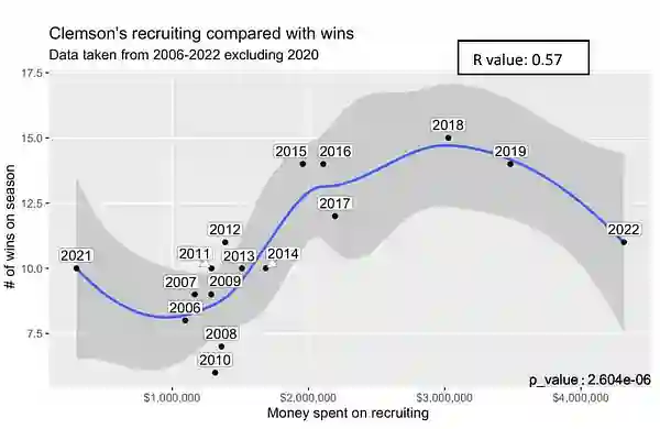
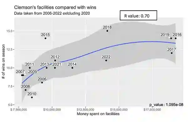
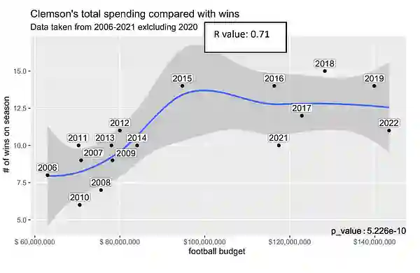
Clemson's football program has grown significantly over the last 20 years. This is evident after their major turnaround in 2011 when they won their first ACC title in 20 years. They started to spend more on recruiting, allowing them to bring in better recruiting classes. This can be seen very clearly in the massive input of cash they put into their facilities in 2012. Clemson quickly turned into one of the most dominant teams in college football. They heavily increased spending after playing in and narrowly losing the national championship for the 2015 season.
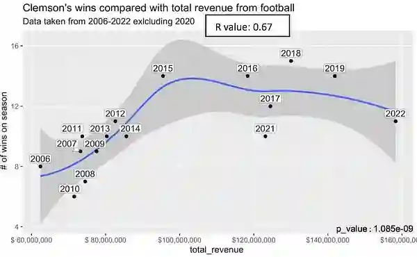
They went on to spend the most money they had ever spent on facilities and won their first national championship in over 35 years after the 2016 season. Clemson’s spending compared to revenue is linear, so the more the program is invested, the greater the return. In one of the most significant investment years in the program financially (2016), there is also a record jump in revenue. While the best financial years weren’t necessarily the winningest seasons, the Revenue and Wins graph does reflect that the national championship seasons built a bigger following, giving better revenue through sales merchandise and advertising for the program.
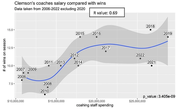
The p-values for each of these graphs on this page (and the graphs looking at these variables for all the other teams in this study) all fell into the statistically significant range, as these relationships appeared to be correlated in a way that was much more likely than would be expected by chance. The R values (the correlation coefficient, which measures the strength of the linear relationship between two quantitative variables) in these graphs show that the effect of spending on facilities on program wins is stronger than the impact of spending on recruiting. Based on this, at least in Clemson’s case, spending on facilities most contributed to their success. The strongest correlation was Total Spending with Revenue. Clemson made significantly more money as they increased spending

Florida State’s Football Spending Analysis
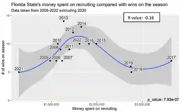
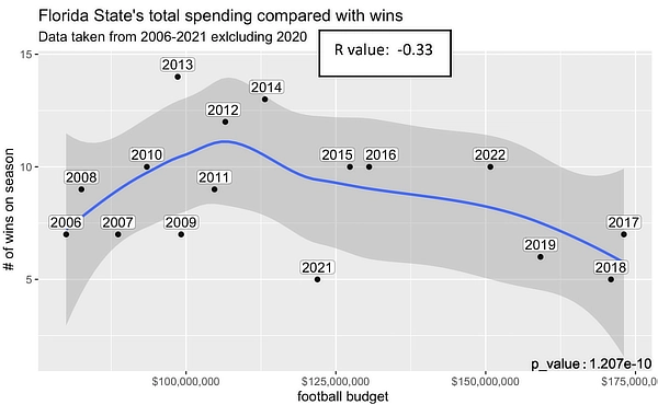
For the last 20 years, Florida State has had the opposite program trajectory of Clemson. They were very successful in the 90s and returned to that level of success in 2013. Their winning started to fizzle out in 2015-2016. Florida State began to spend more money on recruiting after Coach Fisher left, and FSU suffered a less successful season. This is because they lost the ability to recruit many players who wanted to play for Florida State to play under Jimbo Fisher, knowing he was an elite coach.
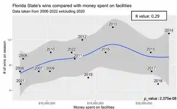
The program has spent less on recruiting due to the smaller revenue made from the past couple of seasons due to a lack of success. The money spent on facilities reached the highest level after their national championship, hoping to reclaim their football dynasty that made up the 90s. Their spending on facilities decreased during the disappointing 2015-2016 years. But then they increased facility spending in 2017 in the hope of helping support the program now under the helm of Willie Taggart. They were trying to establish an image of success by supporting the new head coach, Willie Taggart who would eventually be fired after three years.
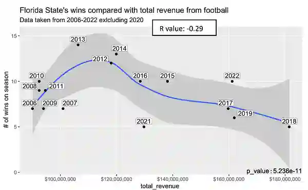
You can see in the fourth graph that despite a drastic decrease in wins through 2017-2019, they still had the highest revenue in program history. This is because the ACC signed a TV deal with ESPN, meaning they got a revenue cut no matter what. This would explain the negative correlation wins had with revenue. Facilities spending correlation with wins was positive, while recruiting expenses was actually a negative correlation with wins during this period.
Alabama Football Spending Analysis
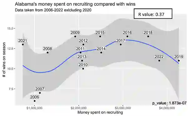
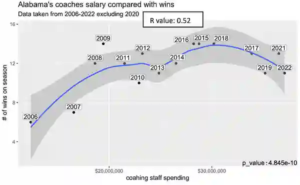
Alabama has been the most dominant program of the last 20 years. They have had six national championship titles since 2006. 2006 was Nick Saban’s first year coaching the Tide. They finished with a 6-7 record. That year was one of the lowest amounts spent on recruiting. You can see a significant jump in 2008, where they averaged more than ten wins a season. After that, there was no looking back. As Alabama began to win more, you could see them gradually invest more into recruiting. There was an exception in 2021; however, this was mainly because Alabama, like many other athletic departments, had to spend less due to its lack of income in 2020.
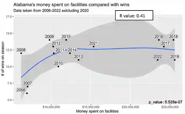
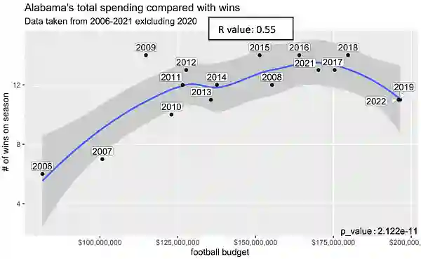
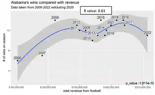
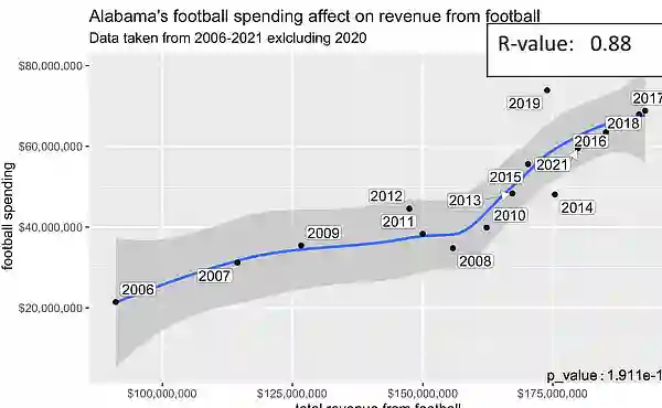
You could see that Alabama’s facilities, too, spent more after a successful 2008 campaign where they went 12-2. Alabama’s revenue was taken to new heights under Saban. They began to spend even more in the playoff era. Clemson started to match their level of success, beating them in the 2016 national championship game. Alabama’s prominence as a football dynasty allowed great ticket sales and lucrative advertisement deals. It also likely increased the value of the SEC deal with ESPN to create the SEC network, a 163-million-dollar agreement in 2014, which has been increasingly renegotiated over the years. Today, each school in the conference makes roughly 49.9 million dollars from the SEC network contract. Alabama's spending linearly affected its revenue share, similar to the other programs.
Looking at the r-value (correlation) and p-value (significance), The strongest correlation between elements besides Spending and Revenue is that of Wins to Income. In years like 2017, when they won their 5th national championship under Saban , they had one of their best revenue years in program history. You could again see that the correlation coefficient and p-value are higher for Facilities Spending, showing that facility spending for football is a more significant driver of wins than Recruiting Spending. However, it also has a positive correlation and a meaningful p-value.
Kansas Football Spending Analysis
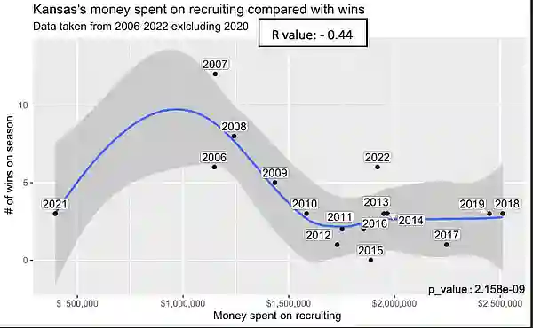
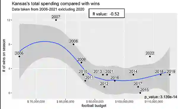
Kansas was the program with the lowest win average since 2006 in this study. Interestingly enough, they had a fantastic 2007 season where they finished 7th in the AP poll. They were close to a shot at the BCS championship. In recruiting, however, winning increased their spending but not significantly. Their head coach, Mark Mingo, was successful but parted ways with the program in 2009. After losing Mingo, Kansas struggled to be bowl eligible until the 2022 season. They did not increase much in recruiting.
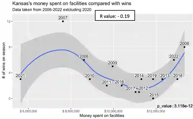
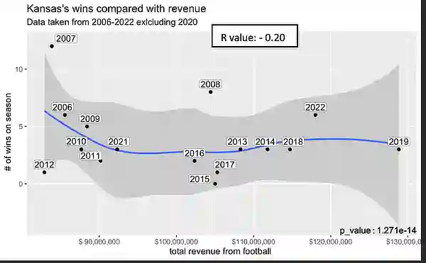
You could see, however, with facilities that they spent their most on the program after their successful 2007 season. However, their facility spending started to stall as they spent a little bit less in 2008. In the Wins compared with Revenue graph, Kansas football revenue grew sharply after their successful season as fans grew, and there was a buzz around the team. As their success tapered, revenue drew back quite a lot.
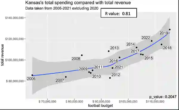
However, they would gradually increase revenue as the Big 12 made a deal with Fox Sports and ESPN in 2012. It was worth over 2.6 billion dollars with a 13-year contract. The Big 12 recently completed a deal for a 2.28-billion-dollar extension for a six-year contract. Kansas’ Revenue and Spending are not very linear, with various moves forward and backward, but it seems recently the program has made the most revenue it has ever made, and are starting to invest in it more.
All the variables negatively correlate to winning. The smallest, however, would be facility spending. This shows that even in a team that struggles to put up a winning season, facility spending helps to impact wins. They have more net revenue than a team like Clemson, who had two national championships during this span. They also had significantly lower spending. This shows how much revenue they could gain from their TV deal.
Texas Football Spending Analysis
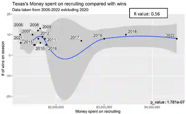
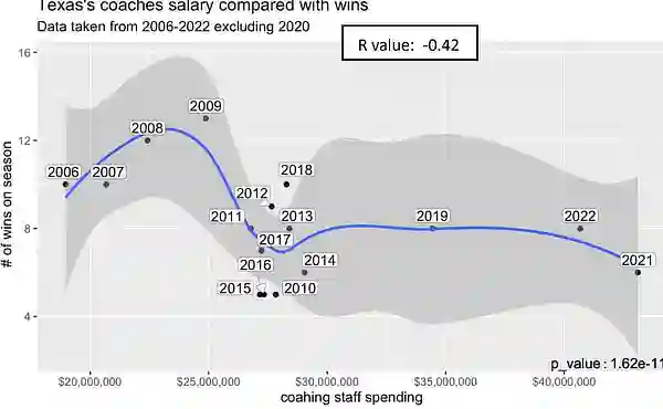
Texas is one of the most recognizable brands in college football. This is partly due to the large market of Texas and the past success that gathered them a large following. Texas already entered the recruiting graph as a high spender because they won the national championship in 2005, so the program was ready to invest more. After some disappointing years, Coach Mac Brown and Texas parted ways in 2013. Texas would bounce around from coach to coach for a while. Recruiting funds were stagnant until 2017.
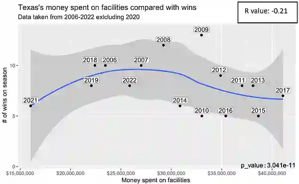
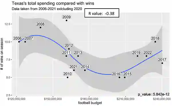
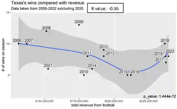
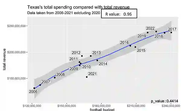
The facilities reached high levels of spending following their national championship appearance in 2009. They would peak in spending in 2017 following their increase in revenue, but they would start to slow down spending in 2018. Texas’ total spending in 2022 rose to a a level that was similar to 2007’s budget. The revenue for Texas reached pretty consistent growth, despite the fact that wins continued to stagnate.
The reason for Texas's growth stemmed from a couple of things. The fact that they were a recognizable brand in a big Texas market helped a lot. They also had their own TV network called the Longhorn Network. Instead of splitting their TV revenue, they got 15 million a year and had deals with ESPN and Fox through the Big 12. This gave them some of the most significant average revenue in college football by over 18 million dollars.
This cash allowed them to spend more than 12 million dollars on average on facilities compared to the team that finished second most on facilities (Ohio State). Texas’ negative correlation for Facility Spending compared with Wins seems to indicate a point of diminishing returns, which was surpassed due to their massive spending on facilities. This also explains why, in Texas’ case, the relationship between Spending on Recruiting and Wins appears stronger than that of Facilities Spending and Wins. Their Spending compared to Wins is still relatively linear, but you can start to see more significant growth from when they had the Longhorn Network in 2011 and when their deals with ESPN and Fox were formed in 2012.As the years progressed, their ESPN Fox Deals became more profitable.
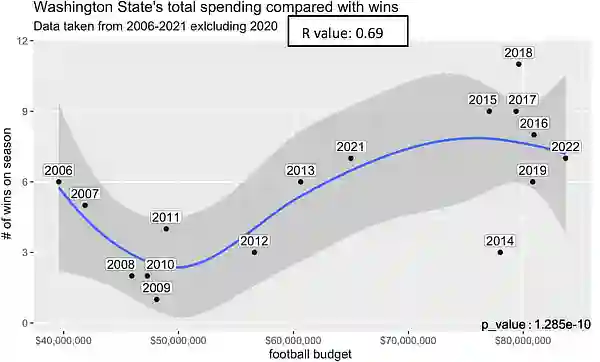
Washington State Football Spending Analysis
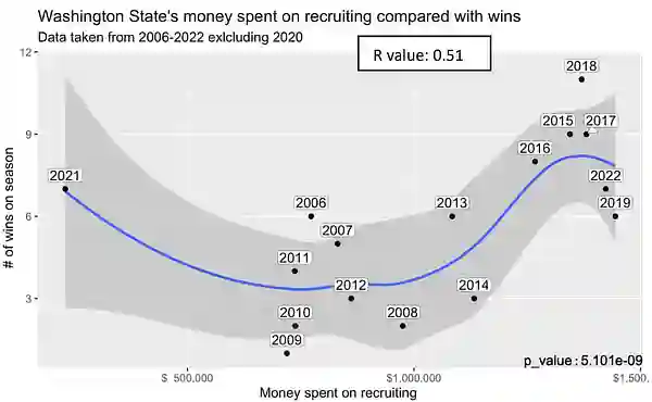
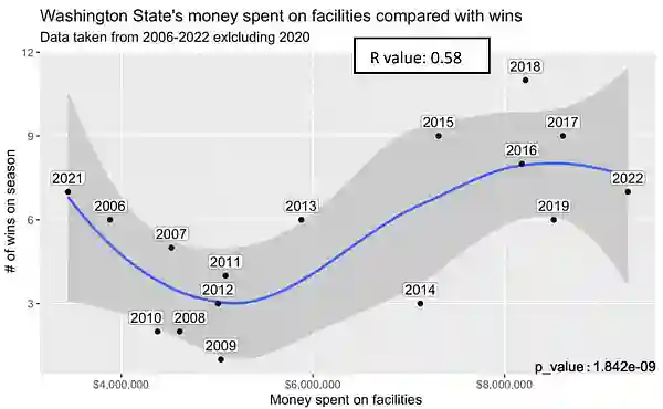
With available data, Washington State had the lowest total spending of any team in all the Power Five. Surprisingly, they did not have the lowest win percentage. WSU began to win more when Mike Leach became the head coach in 2012 and gained success in 2013. They also increased levels of Recruiting and Facility Spending under Coach Leach. However, the Facility Spending was closer to other teams' averages than the money spent on recruiting.
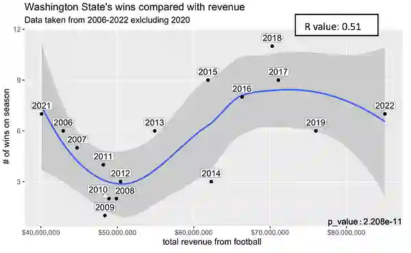
Predictably, as shown in the fourth graph, 2013 was a tremendous jump in Revenue due to their winningest season since 2006. Leach led an air raid offense that passed heavily with constant looks down the field. This brought more attention to the games and allowed them to prevail against Pac-12 defenses who weren’t yet used to this new offensive look. While Washington State did make more money during their more successful years with Leach, they still earned the least revenue of all the teams with available data.
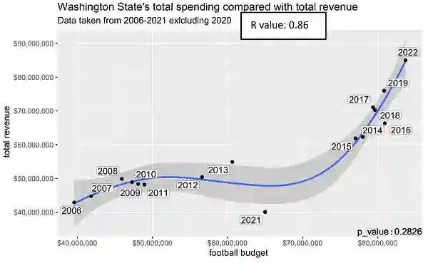
They are now hoping to find success with their new head coach, Jake Dickert, the 39-year-old former defensive coordinator at Wyoming. There could be a couple of reasons for their financial shortcomings: It is on the east side of Washington, far from the closest big markets in the Northwest (Seattle and Portland). Both of those cities, for the most part, follow Washington and Oregon’s football teams. Another reason for their small revenue is that they have the fourth most minor TV deal out of the power conferences. However, you can see their spending and income were pretty linear. Their most robust correlation coefficient was Revenue to Spending. This shows that the variable of Facilities Spending had the most substantial chance of increasing wins.
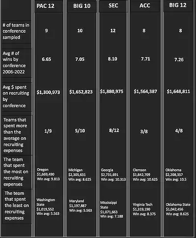
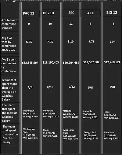
Average spent on recruiting among Power 5 Conferences
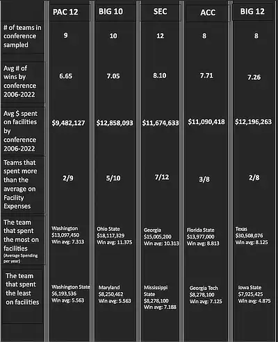
Average spent on facilities among Power 5 Conferences
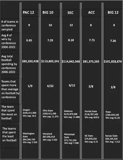
Average total spending among Power 5 Conferences
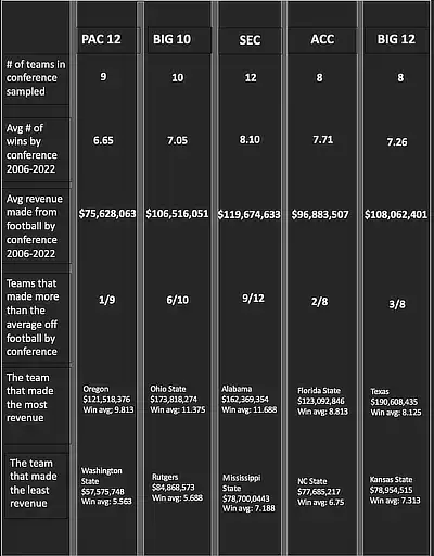
Average revenue generated among Power 5 Conferences
Average spending on coaching among Power 5 Conferences
Comparing recruiting and wins from all available data
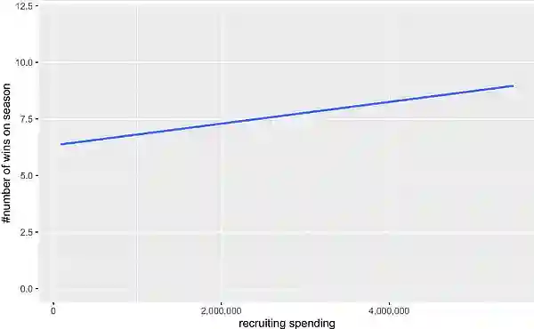
Using a Generalized Additive Model (GAM) allows us to model the relationship between Spending on Recruiting and Wins in football teams. The GAM allows for non-linear relationships between the predictor and the response variable.
The estimated coefficient for the intercept is 7.3337. The intercept represents the expected wins when the recruiting metrics are zero. With a standard error of 0.1021, which calculates the likelihood of correctly representing the population, the lower to zero, the more accurate it is. The intercept represents the expected wins when the recruiting metrics are zero. The p-value is 2.31e-07, indicating that the smooth term is statistically significant. The adjusted R-squared value for the model is 0.0379, indicating that the recruiting metrics can explain approximately 3.79% of the variance in the wins.
What this means:
The analysis reveals a statistically significant relationship between Recruiting Spending and wins in Power Five football teams. The GAM model indicates a non-linear relationship between the two variables. However, the adjusted R-squared value suggests that Recruiting Spending explains only a small portion (3.79%) of the variance in the number of wins.
Comparing facilities and wins from all available data
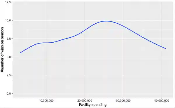
The estimated coefficient for the intercept is 7.33374. The intercept represents the expected wins when the facilities metric is zero. The standard error of 0.09907, with an even lower showing, represents the data better than the previous graph. The p-value is <2e-16, indicating that the smooth term is highly statistically significant. The adjusted R-squared value for the model is 0.0941, meaning that the facilities metric can explain approximately 9.41% of the variance is the number of wins.
What this means:
The analysis reveals a statistically significant non-linear relationship between facilities and wins in Power Five football teams. Facilities Spending explains approximately 9.41% of the variance in the number of Wins. This suggests that the quality and condition of a team's facilities play a significant role in its performance and success on the field.
Comparing total spending and wins from all available data
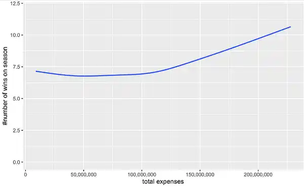
The estimated coefficient for the intercept is 7.3896. The intercept represents the expected number of wins when total expenses are zero. The standard error of 0.1047, its low value, shows that the smoothed data represents the population well. The P-value is <2e-16, indicating that the smooth term is highly statistically significant. The adjusted R-squared value for the model is 0.0712, which means that approximately 7.12% of the variance in the number of wins can be explained by total Spending.
What this means:
The analysis reveals a statistically significant non linear relationship between total expenses and wins in Power Five football teams. Total Spending explains approximately 7.12% of the variance in the number of Wins.
Comparing revenue and wins from all available data
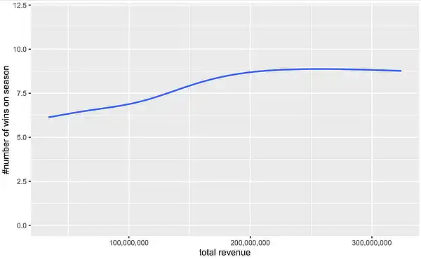
The estimated coefficient for the intercept is 109,014,287. The intercept represents the expected revenue when there are no wins. The p-value is <2e-16, indicating that the smooth term is statistically significant. The adjusted R-squared value for the model is 0.084, which means that approximately 8.4% of the variance in the revenue can be explained by wins.
What this means:
The analysis reveals a statistically significant non-linear relationship between total Revenue and Wins in Power Five football teams. The number of Wins explains approximately 8.4% of the variance in the Total Revenue. Total Spending compared with Revenue.
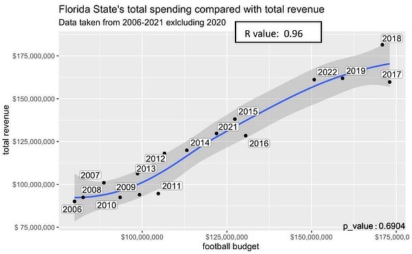
Comparing spending and revenue from all available data
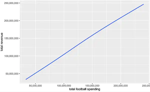
The estimated coefficient for the intercept is 107,833,159. The intercept represents the expected total revenue when total expenses are zero. The p-value is <2e-16, indicating that the smooth term is highly statistically significant. The adjusted R-squared value for the model is 0.868, which means that approximately 86.8% of the variance in total revenue can be explained by total expenses.
What this means:
The analysis reveals a statistically significant non-linear relationship between total expenses and total revenue in Power Five football teams. Total Spending explains approximately 86.8% of the variance in total Revenue.
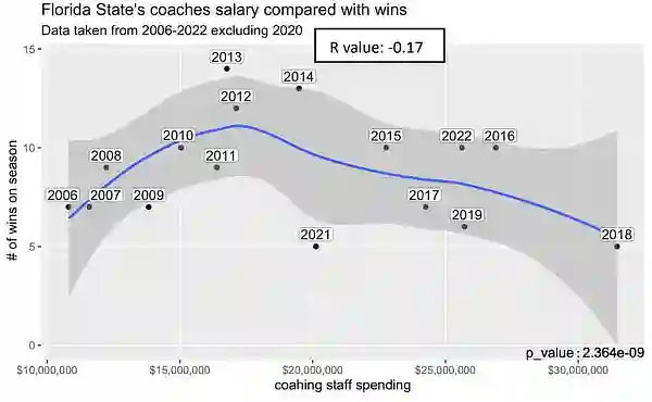
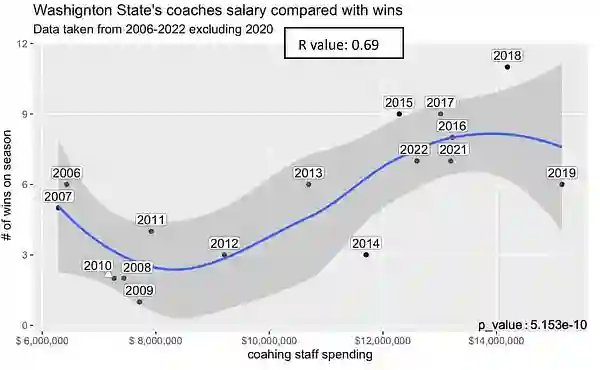
Comparing spending on coaches and wins from all available data
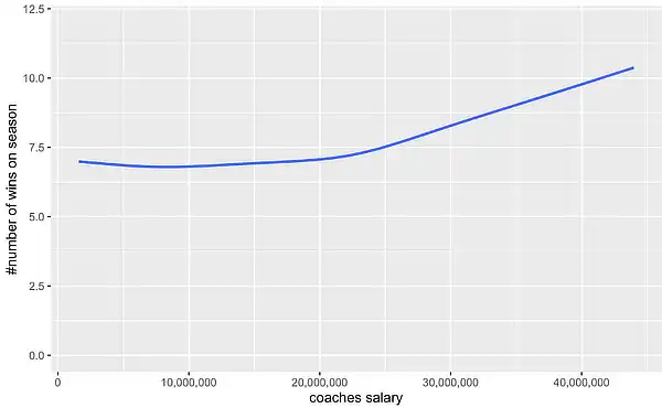
The estimated coefficient for the intercept is 7.3896. The intercept represents the expected number of wins when coach spending is zero. With the standard error of 0.1045, the smooth data is represented well. The adjusted R-squared value for the model is 0.0749, which means that about 7.49% of the variance in the number of wins can be explained by coach spending.
What this means:
The analysis reveals a statistically significant non-linear relationship between coach spending and wins in Power Five football teams. Coaches’ Spending explains approximately 7.49% of the variance in the number of Wins.
Conclusions:
One of the main takeaways is that a significant positive correlation often exists between wins and football spending.
- The correlation between football spending and revenue has the strongest correlation.
Texas spent the most and made the most even though they were not the winningest team. The reasons for this are that successful seasons take time for a following to consistently back the team, which will take longer to show an evident growth in revenue than just one year. Plus, the massive TV deals signed by conferences and TV networks make a large portion of the income, and each team in the conference gets the same pay cut regardless of record. Wins do matter, though, as the TV deals are more lucrative for conferences with more successful teams and larger followings.
- Most teams had a stronger correlation between Wins and Revenue than the relationship between Spending and Wins. Teams that had long-term success in revenue and who won consistently spent more and more money each season, having to compete to maintain their level of success rather than staying complacent with their spending.
There was also a trend that teams with coaching changes would often have a poor transition year, which resulted in the athletics department cutting back on football spending - creating difficulties for the new coach when recruiting big-time players to their school. A team that bucked this trend was Alabama. Despite having a disappointing 6-6 season in Saban’s first year with Alabama, they didn’t cut spending - allowing him to build a program that maintained success.
- Most of the time, money spent on facilities (a form of recruiting) correlates more significantly to wins than money spent on other forms of recruiting and coaches' visits.
- The last thing to gain from this is the TV deal's effects on the school's revenue from their football program. These TV contracts lead to significant increases in Revenue, allowing for greater Spending. Teams without these deals are at a considerable disadvantage regarding their spending ability, which we have shown is related to future revenue and wins.
Sources
Knight Commission on intercollegiate athletics. (n.d.). Knight-Newhouse College Athletics Database, a joint project of the Knight Commission on Intercollegiate Athletics and the S.I. Newhouse School of Public Communications, Syracuse University. College Athletics Database.
ESPN Internet Ventures. (n.d.). NCAA on ESPN - college football scores, stats and highlights. ESPN. https://www.espn.com/college-football
I, Christian Haworth, permit for this photo to be used article_cover page_heic in the article
About the Author
 Christian Haworth is an Economics major in the sports analytics program at Samford.